Melt Plumes

The documentation starts with the nuts and bolts. If you want to skip some details, go straight to the section Simple Solver Interface below.

Quick Start

import numpy as np
import matplotlib.pyplot as plt
import scipy.integrate as itgr
import melt_plumes.bpt as bpt
import seawater as sw

/home/runner/work/melt-plumes/melt-plumes/src/melt_plumes/bpt.py:3: UserWarning: The seawater library is deprecated! Please use gsw instead.
  import seawater as sw

Plume in a homogeneous ocean

Set up ocean conditions for line plume. Below we use constant temperature and salinity ocean.

d = np.arange(1.0, 201.0, 1.0)  # Depths (m)
T = 15.0  # (degree_C)
S = 25.0  # (PSU)

# Initial conditions
W = 100  # Channel width (m)
Q = 50.0  # Discharge rate (m3 s-1)
α = 0.1  # Entrainment coefficient
lat = 60.0  # Latitude
zi = -180  # Starting height (m)
ρ_0 = 1025  # Density constant (kg m-3)
g = -9.81  # Gravity (m s-2)
Si = 0.0000001  # Need a small initial salinity apparently!
u = 0.0  # Background horizontal ocean velocity (m s-1)

# Derived initial conditions
Qm2s = Q / W  # Discharge rate per m (m2 s-1)
pi = sw.pres(-zi, lat)  # Pressure (dbar)
Ti = sw.fp(Si, pi)  # Temperature is the freezing point (C)
ρi = sw.pden(S, T, pi, pr=0)  # Far-field ocean density (kg m-3)
ρ_oi = sw.pden(Si, Ti, pi, pr=0)  # Plume density (kg m-3)
gpi = g * (ρ_oi - ρi) / ρ_0  # Reduced gravity (m s-2)
# Vertical velocity (m s-1), from balance of momentum and buoyancy for a line plume
wi = (gpi * Qm2s / α) ** (1 / 3)
Ri = Qm2s / wi  # Radius or thickness (m)

mass_flux = Qm2s  # Mass flux (m2 s-1)
mom_flux = Qm2s * wi  # Momentum flux (m3 s-2)
T_flux = Qm2s * Ti  # Temperature flux (C m2 s-1)
S_flux = Qm2s * Si  # Salt flux (PSU m2 s-1)

fluxes0 = [mass_flux, mom_flux, T_flux, S_flux]
args = (T, S, u, α, ρ_0, g, lat)

z_eval = np.arange(zi, -d[0], 1)

result = itgr.solve_ivp(
    bpt.bpt,
    [zi, -d[0]],
    fluxes0,
    method="RK45",
    t_eval=z_eval,
    args=args,
    events=bpt.Δρ,
)

mass_flux = result.y[0, :]
mom_flux = result.y[1, :]
T_flux = result.y[2, :]
S_flux = result.y[3, :]

w = mom_flux / mass_flux  # Plume vertical velocity (m s-1)
R = mass_flux / w  # Plume thickness or radius (m)
T_o = T_flux / mass_flux  # Plume temperature (C)
S_o = S_flux / mass_flux  # Plume salinity (PSU)

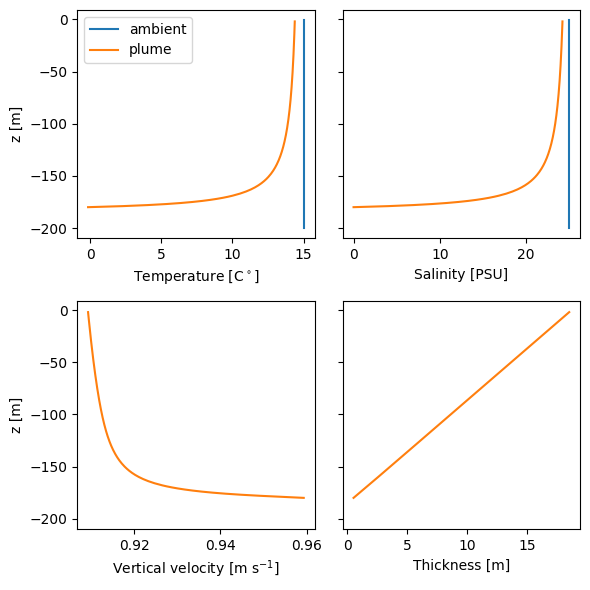
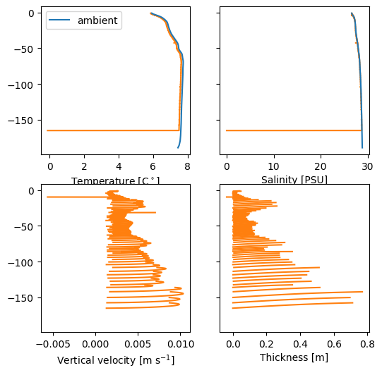
The plume theory equations describe fluxes of quantities such as momentum and buoyancy. Typical measureable quantities such as velocity and temperature are derived from the fluxes. Below we plot the results.

z_out = result.t

fig, axs = plt.subplots(2, 2, figsize=(6, 6), sharey=True)

axs[0, 0].plot(np.full_like(d, T), -d, label="ambient")
axs[0, 0].plot(T_o, z_out, label="plume")
axs[0, 0].set_xlabel("Temperature [C$^\circ$]")
axs[0, 0].legend()

axs[0, 1].plot(np.full_like(d, S), -d)
axs[0, 1].plot(S_o, z_out)
axs[0, 1].set_xlabel("Salinity [PSU]")

axs[1, 0].plot(w, z_out, "C1")
axs[1, 0].set_xlabel("Vertical velocity [m s$^{-1}$]")

axs[1, 1].plot(R, z_out, "C1")
axs[1, 1].set_xlabel("Thickness [m]")

for ax in axs[:, 0]:
    ax.set_ylabel("z [m]")

fig.tight_layout()

<>:7: SyntaxWarning: invalid escape sequence '\c'
<>:7: SyntaxWarning: invalid escape sequence '\c'
/tmp/ipykernel_2201/588080408.py:7: SyntaxWarning: invalid escape sequence '\c'
  axs[0, 0].set_xlabel("Temperature [C$^\circ$]")

Plumes in realistic stratification

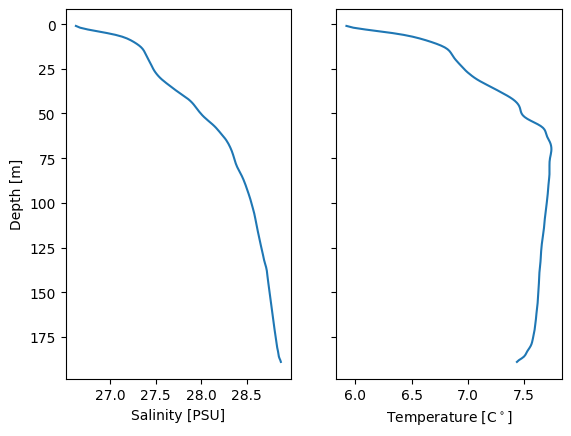
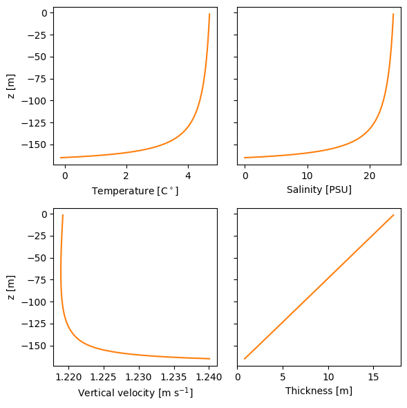
The melt-plumes package contains some data from a fjord in Alaska (LeConte Bay or Xeitl Sit’ in Tlingit).

from melt_plumes import helpers

d, S, T = helpers.load_LeConte_CTD()

fig, axs = plt.subplots(1, 2, sharey=True)
axs[0].plot(S, d)
axs[1].plot(T, d)
axs[0].invert_yaxis()
axs[0].set_ylabel("Depth [m]")
axs[0].set_xlabel("Salinity [PSU]")
axs[1].set_xlabel("Temperature [C$^\circ$]")

<>:11: SyntaxWarning: invalid escape sequence '\c'
<>:11: SyntaxWarning: invalid escape sequence '\c'
/tmp/ipykernel_2201/2474716005.py:11: SyntaxWarning: invalid escape sequence '\c'
  axs[1].set_xlabel("Temperature [C$^\circ$]")

Text(0.5, 0, 'Temperature [C$^\\circ$]')

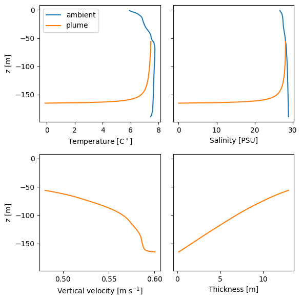
Use interp1d to generate a function that linearly interpolates the data between observed depths. The buoyant plume theory equations can then be solved using this interpolating function.

import scipy.interpolate as itpl

Sz = itpl.interp1d(-d, S)
Tz = itpl.interp1d(-d, T)

# Initial conditions
W = 100  # Channel width (m)
Q = 10.0  # Discharge rate (m3 s-1)
α = 0.1  # Entrainment coefficient
lat = 60.0  # Latitude
zi = -165  # Height (m)
ρ_0 = 1025  # Density constant (kg m-3)
g = -9.81  # Gravity (m s-2)
Si = 0.0000001  # Need a small initial salinity apparently!
u = 0.0  # Background horizontal ocean velocity (m s-1)

# Derived
Qm2s = Q/W  # Discharge rate per m (m2 s-1)
pi = sw.pres(-zi, lat)  # Pressure (dbar)
Ti = sw.fp(Si, pi)  # Temperature is the freezing point (C)
ρi = sw.pden(Sz(zi), Tz(zi), pi, pr=0)  # Far-field ocean density (kg m-3)
ρ_oi = sw.pden(Si, Ti, pi, pr=0)  # Plume density (kg m-3)
gpi = g * (ρ_oi - ρi) / ρ_0  # Reduced gravity (m s-2)
wi = (gpi * Qm2s / α)**(1/3)  # Vertical velocity (m s-1), from balance of momentum and buoyancy for a line plume
Ri = Qm2s / wi  # Radius or thickness (m)

mass_flux = Qm2s  # Mass flux (m2 s-1)
mom_flux = Qm2s * wi  # Momentum flux (m3 s-2)
T_flux = Qm2s * Ti  # Temperature flux (C m2 s-1)
S_flux = Qm2s * Si  # Salt flux (PSU m2 s-1)

fluxes0 = [mass_flux, mom_flux, T_flux, S_flux]
args = (Tz, Sz, u, α, ρ_0, g, lat)

z_eval = np.arange(zi, -d[0], 1)

result = itgr.solve_ivp(
    bpt.bpt,
    [zi, -d[0]],
    fluxes0,
    method="RK45",
    t_eval=z_eval,
    args=args,
    events=bpt.Δρ,
)

mass_flux = result.y[0, :]
mom_flux = result.y[1, :]
T_flux = result.y[2, :]
S_flux = result.y[3, :]

w = mom_flux / mass_flux  # Plume vertical velocity (m s-1)
R = mass_flux / w  # Plume thickness or radius (m)
T_o = T_flux / mass_flux  # Plume temperature (C)
S_o = S_flux / mass_flux  # Plume salinity (PSU)

z_out = result.t

fig, axs = plt.subplots(2, 2, figsize=(6, 6), sharey=True)

axs[0, 0].plot(T, -d, label="ambient")
axs[0, 0].plot(T_o, z_out, label="plume")
axs[0, 0].set_xlabel("Temperature [C$^\circ$]")
axs[0, 0].legend()

axs[0, 1].plot(S, -d)
axs[0, 1].plot(S_o, z_out)
axs[0, 1].set_xlabel("Salinity [PSU]")

axs[1, 0].plot(w, z_out, "C1")
axs[1, 0].set_xlabel("Vertical velocity [m s$^{-1}$]")

axs[1, 1].plot(R, z_out, "C1")
axs[1, 1].set_xlabel("Thickness [m]")

for ax in axs[:, 0]:
    ax.set_ylabel("z [m]")

fig.tight_layout()

<>:7: SyntaxWarning: invalid escape sequence '\c'
<>:7: SyntaxWarning: invalid escape sequence '\c'
/tmp/ipykernel_2201/3723151647.py:7: SyntaxWarning: invalid escape sequence '\c'
  axs[0, 0].set_xlabel("Temperature [C$^\circ$]")

A chain of plumes

Loop over the prior exmaple.

from textwrap import dedent

results = []

# Initial conditions
W = 1000  # Channel width (m)
Q = 0.000001  # Discharge rate (m3 s-1)
α = 0.1  # Entrainment coefficient
lat = 60.0  # Latitude
zi = -165  # Height (m)
ρ_0 = 1025  # Density constant (kg m-3)
g = -9.81  # Gravity (m s-2)
Si = 1e-8  # Need a small initial salinity apparently!
u = 0.0  # Background horizontal ocean velocity (m s-1)
n_plumes_max = 1000  # Maximum number of plumes
dz = 0.1  # solver evaluation spacing (m)

# Derived
Qm2s = Q/W  # Discharge rate per m (m2 s-1)
pi = sw.pres(-zi, lat)  # Pressure (dbar)
Ti = sw.fp(Si, pi)  # Temperature is the freezing point (C)
ρi = sw.pden(Sz(zi), Tz(zi), pi, pr=0)  # Far-field ocean density (kg m-3)
ρ_oi = sw.pden(Si, Ti, pi, pr=0)  # Plume density (kg m-3)
gpi = g * (ρ_oi - ρi) / ρ_0  # Reduced gravity (m s-2)
wi = (gpi * Qm2s / α)**(1/3)  # Vertical velocity (m s-1), from balance of momentum and buoyancy for a line plume
Ri = Qm2s / wi  # Radius or thickness (m)

mass_flux = Qm2s  # Mass flux (m2 s-1)
mom_flux = Qm2s * wi  # Momentum flux (m3 s-2)
T_flux = Qm2s * Ti  # Temperature flux (C m2 s-1)
S_flux = Qm2s * Si  # Salt flux (PSU m2 s-1)

args = (Tz, Sz, u, α, ρ_0, g, lat)
fluxes0 = [mass_flux, mom_flux, T_flux, S_flux]

z_eval = np.arange(zi, -d[0] - dz/2, dz)

for n_plumes in range(1, n_plumes_max+1):

    result = itgr.solve_ivp(
        bpt.bpt,
        [zi, -d[0]],
        fluxes0,
        method="RK45",
        t_eval=z_eval,
        args=args,
        events=bpt.Δρ,
    )

    results.append(result)

    if np.isclose(result.t[-1], -d[0] - dz):

        text = f"""
        Number of plumes = {n_plumes}
        Starting height of last plume = {zi:1.2f}  m
        """

        print(dedent(text))

        break

    zi = result.t_events[0][0]

    Qm2s = Q/W  # Discharge rate per m (m2 s-1)
    pi = sw.pres(-zi, lat)  # Pressure (dbar)
    Ti = sw.fp(Si, pi)  # Temperature is the freezing point (C)
    ρi = sw.pden(Sz(zi), Tz(zi), pi, pr=0)  # Far-field ocean density (kg m-3)
    ρ_oi = sw.pden(Si, Ti, pi, pr=0)  # Plume density (kg m-3)
    gpi = g * (ρ_oi - ρi) / ρ_0  # Reduced gravity (m s-2)
    wi = (gpi * Qm2s / α)**(1/3)  # Vertical velocity (m s-1), from balance of momentum and buoyancy for a line plume
    Ri = Qm2s / wi  # Radius or thickness (m)

    mass_flux = Qm2s  # Mass flux (m2 s-1)
    mom_flux = Qm2s * wi  # Momentum flux (m3 s-2)
    T_flux = Qm2s * Ti  # Temperature flux (C m2 s-1)
    S_flux = Qm2s * Si  # Salt flux (PSU m2 s-1)
    fluxes0 = [mass_flux, mom_flux, T_flux, S_flux]

    z_eval = np.arange(np.ceil(zi / dz) * dz, -d[0] - dz/2, dz)

Number of plumes = 94
Starting height of last plume = -1.54  m

fig, axs = plt.subplots(2, 2, figsize=(6, 6), sharey=True)

for result in results:
    mass_flux = result.y[0, :]
    mom_flux = result.y[1, :]
    T_flux = result.y[2, :]
    S_flux = result.y[3, :]
    w = mom_flux / mass_flux  # Plume vertical velocity (m s-1)
    R = mass_flux / w  # Plume thickness or radius (m)
    T_o = T_flux / mass_flux  # Plume temperature (C)
    S_o = S_flux / mass_flux  # Plume salinity (PSU)
    z_out = result.t

    axs[0, 0].plot(T_o, z_out, "C1")
    axs[0, 0].set_xlabel("Temperature [C$^\circ$]")

    axs[0, 1].plot(S_o, z_out, "C1")
    axs[0, 1].set_xlabel("Salinity [PSU]")

    axs[1, 0].plot(w, z_out, "C1")
    axs[1, 0].set_xlabel("Vertical velocity [m s$^{-1}$]")

    axs[1, 1].plot(R, z_out, "C1")
    axs[1, 1].set_xlabel("Thickness [m]")

axs[0, 0].plot(T, -d, "C0", label="ambient")
axs[0, 1].plot(S, -d, "C0")
axs[0, 0].legend()

<>:15: SyntaxWarning: invalid escape sequence '\c'
<>:15: SyntaxWarning: invalid escape sequence '\c'
/tmp/ipykernel_2201/3450213895.py:15: SyntaxWarning: invalid escape sequence '\c'
  axs[0, 0].set_xlabel("Temperature [C$^\circ$]")

<matplotlib.legend.Legend at 0x7f0fe25b4e90>

Simple solver interface

from melt_plumes import solve

w, R, T_o, S_o, z_out = solve.plume(-165, 100, 0.5)

fig, axs = plt.subplots(2, 2, figsize=(6, 6), sharey=True)

axs[0, 0].plot(T_o, z_out, "C1", label="plume")
axs[0, 0].set_xlabel("Temperature [C$^\circ$]")

axs[0, 1].plot(S_o, z_out, "C1")
axs[0, 1].set_xlabel("Salinity [PSU]")

axs[1, 0].plot(w, z_out, "C1")
axs[1, 0].set_xlabel("Vertical velocity [m s$^{-1}$]")

axs[1, 1].plot(R, z_out, "C1")
axs[1, 1].set_xlabel("Thickness [m]")

for ax in axs[:, 0]:
    ax.set_ylabel("z [m]")

fig.tight_layout()

<>:8: SyntaxWarning: invalid escape sequence '\c'
<>:8: SyntaxWarning: invalid escape sequence '\c'
/tmp/ipykernel_2201/1914993096.py:8: SyntaxWarning: invalid escape sequence '\c'
  axs[0, 0].set_xlabel("Temperature [C$^\circ$]")

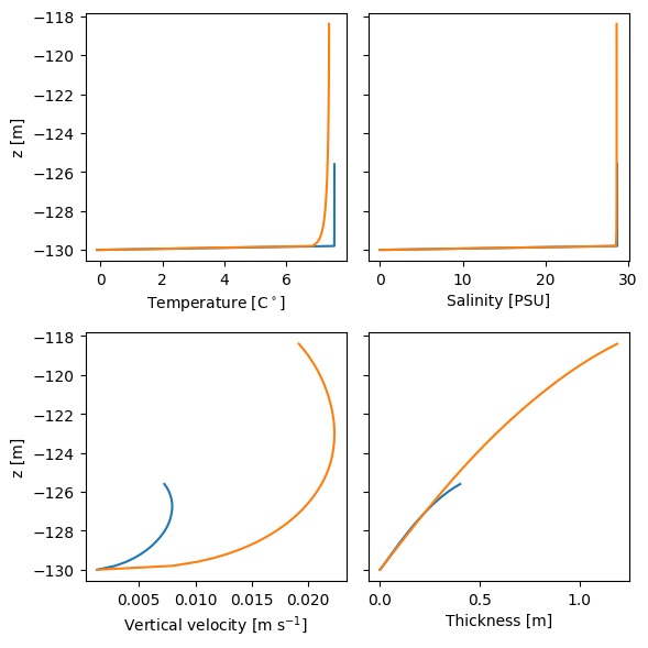
Ambient plume with and without horizontal velocity

fig, axs = plt.subplots(2, 2, figsize=(6, 6), sharey=True)

w, R, T_o, S_o, z_out = solve.plume(-130, 0.0000001, 0.2, T=Tz, S=Sz, u=0.0)
w_u, R_u, T_o_u, S_o_u, z_out_u = solve.plume(-130, 0.0000001, 0.2, T=Tz, S=Sz, u=0.05)

axs[0, 0].plot(T_o, z_out, label="")
axs[0, 0].plot(T_o_u, z_out_u, label="+u")
axs[0, 0].set_xlabel("Temperature [C$^\circ$]")

axs[0, 1].plot(S_o, z_out)
axs[0, 1].plot(S_o_u, z_out_u)
axs[0, 1].set_xlabel("Salinity [PSU]")

axs[1, 0].plot(w, z_out)
axs[1, 0].plot(w_u, z_out_u)
axs[1, 0].set_xlabel("Vertical velocity [m s$^{-1}$]")

axs[1, 1].plot(R, z_out)
axs[1, 1].plot(R_u, z_out_u)
axs[1, 1].set_xlabel("Thickness [m]")

for ax in axs[:, 0]:
    ax.set_ylabel("z [m]")

fig.tight_layout()

<>:8: SyntaxWarning: invalid escape sequence '\c'
<>:8: SyntaxWarning: invalid escape sequence '\c'
/tmp/ipykernel_2201/1577880902.py:8: SyntaxWarning: invalid escape sequence '\c'
  axs[0, 0].set_xlabel("Temperature [C$^\circ$]")

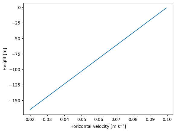
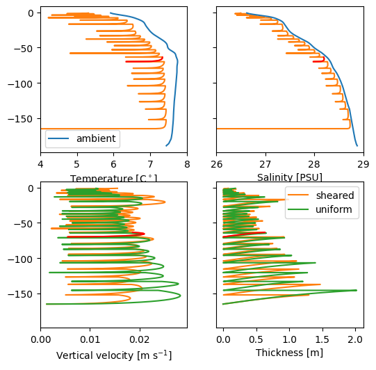
Plume chain with nonuniform horizontal velocity

# Linear velocity profile
def u(z, u0, uzmin, zmin):
    dudz = (uzmin - u0)/zmin
    return dudz*z + u0

uz = lambda z: u(z, 0.1, 0.02, -165)

w, R, T_o, S_o, z_out, idx = solve.plume_chain(-165, 0.000001, 0.1, T=Tz, S=Sz, u=uz, W=1000)

# Comopare to constant velocity case
w_const, R_const, _, _, z_out_const, _ = solve.plume_chain(-165, 0.000001, 0.1, T=Tz, S=Sz, u=0.06, W=1000)

Number of plumes = 24
Starting height of last plume = -2.09  m

Number of plumes = 25
Starting height of last plume = -3.05  m

fig, ax = plt.subplots()
ax.plot(uz(z_out), z_out)
ax.set_xlabel("Horizontal velocity [m s$^{-1}$]")
ax.set_ylabel("Height [m]")

fig, axs = plt.subplots(2, 2, figsize=(6, 6), sharey=True)

axs[0, 0].plot(T_o, z_out, "C1")
axs[0, 0].plot(T_o[idx == 10], z_out[idx == 10], "red")
axs[0, 0].set_xlabel("Temperature [C$^\circ$]")
axs[0, 0].set_xlim(4, 8)

axs[0, 1].plot(S_o, z_out, "C1")
axs[0, 1].plot(S_o[idx == 10], z_out[idx == 10], "red")
axs[0, 1].set_xlabel("Salinity [PSU]")
axs[0, 1].set_xlim(26, 29)

axs[1, 0].plot(w, z_out, "C1")
axs[1, 0].plot(w_const, z_out_const, "C2")
axs[1, 0].plot(w[idx == 10], z_out[idx == 10], "red")
axs[1, 0].set_xlabel("Vertical velocity [m s$^{-1}$]")

axs[1, 1].plot(R, z_out, "C1", label="sheared")
axs[1, 1].plot(R_const, z_out_const, "C2", label="uniform")
axs[1, 1].plot(R[idx == 10], z_out[idx == 10], "red")
axs[1, 1].set_xlabel("Thickness [m]")

axs[0, 0].plot(T, -d, "C0", label="ambient")
axs[0, 1].plot(S, -d, "C0")
axs[0, 0].legend()
axs[1, 1].legend()

<>:10: SyntaxWarning: invalid escape sequence '\c'
<>:10: SyntaxWarning: invalid escape sequence '\c'
/tmp/ipykernel_2201/1328383204.py:10: SyntaxWarning: invalid escape sequence '\c'
  axs[0, 0].set_xlabel("Temperature [C$^\circ$]")

<matplotlib.legend.Legend at 0x7f0fe1dbede0>

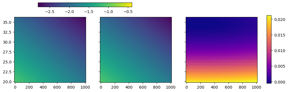
The freezing point approximation

d = np.linspace(0, 1000, 50)
S = np.linspace(20, 36, 30)

fpmin = -2.8
fpmax = -0.4

dg, Sg = np.meshgrid(d, S)

Tlinear = bpt.fp(-dg, Sg)

Teos80 = sw.fp(Sg, sw.pres(dg, 60))

fig, axs = plt.subplots(1, 3, sharex=True, sharey=True, figsize=(11, 3))
PC0 = axs[0].pcolormesh(dg, Sg, Teos80, vmin=fpmin, vmax=fpmax)
axs[1].pcolormesh(dg, Sg, Tlinear, vmin=fpmin, vmax=fpmax)
PC1 = axs[2].pcolormesh(dg, Sg, Tlinear - Teos80, cmap="plasma")

plt.colorbar(PC0, cax=fig.add_axes((0.2, 1.0, 0.3, 0.05)), orientation="horizontal")
plt.colorbar(PC1, cax=fig.add_axes((0.93, 0.1, 0.015, 0.8)))
    

<matplotlib.colorbar.Colorbar at 0x7f0fe28bc5c0>